|
|
| SERVIR:
Central America & Caribbean- CI Nowcasting
6.5-10.7
um Temporal Trends
As described in the "Infrared Products Description" section, the 6.5-10.7 um band difference is useful for inferring cloud top height. The images above provide examples of temporal trends in this band subtraction technique. Values of this band subtraction technique typically range from around -50 to +3 K. The highest (postive) values of this technique indicate the presence of high clouds at or above ("over-shooting" cumulus tops) the tropopause whereas the lowest (negative) values are indicative of clear sky. Therefore, the highest temporal change in this technique can be +/- 53 K. A highly negative (-20 or greater) temporal change indicates one of two things: 1) high cloud movement away from a location (currently negative - formerly postive = negative value) or 2) rapid high cloud decay (currently highly negative - formerly slightly negative (positive) = negative value). A highly positive value can also mean one of two things: 1) high cloud movement into a location (i.e. cirrus expansion, currently positive - formerly negative = positive value) or 2) cumulus growth. Cumulus growth is what we are most interested in determining. Trend values of 3 K/15 mins were found to precede CI in several CI events syudied in the development of the CI nowcast algorithm. Hence, this value is used as an interest field for CI nowcasting. (back to top-->) 13.3-10.7
um Temporal Trends
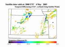
As described in the "Infrared Products Description" section, the 13.3-10.7 um band difference is useful for inferring cloud height and cloud type. The image above provides an example of the 30 min temporal trend in this band subtraction technique. Values of this band subtraction technique typically range from around -30 to +3 K. The highest (postive) values of this technique indicate the presence of high cirrus or mature cumulus clouds whereas the lowest (negative) values are indicative of low clouds such as immature cumulus, stratus, and fog. Therefore, the highest temporal change in this technique can be +/- 33 K. A highly negative temporal change indicates cirrus expansion (currently negative - formerly postive (or 0)= negative value). A positive value indicates cumulus growth. (currently positive - formerly negative (or 0) = positive value) Trend values of 3 K/15 mins were also found to precede CI in several CI events syudied in the development of the CI nowcast algorithm. Hence, this value is used as an interest field for CI nowcasting. (back to top-->) 10.7
um Temporal Trends
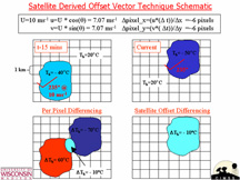
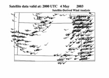
This technique, documented in Roberts and Rutledge (2003), involves examination of time trends in 10.7 um TB (cloud top temp.). In this work, the authors noted that "the onset of vigorous cloud growth leading to storm development was characterized by cloud tops that reached sub-freezing temperatures and exhibited large cooling rates at cloud top 15 min. prior to the first detection of 10 dBZ radar echoes aloft and 30 min before 35 dBZ. The rate of cloud top temperature change was found to be important for descriminating between weakly precipitating storms (<35 dBZ) and vigorous convective storms (>35 dBZ)." The cloud top cooling rate for "weak, limited growth" was 4 K/15 mins and was 8 K/15 mins for "vigorous" growth. The product above illustrates locations exhibitng "weak, limited" growth" (i.e. the 4 K/15 mins threshold). We utilized the "satellite-derived offset vector" technique (described above) to perform the cloud top trend estimates. We have also calculated the cloud top cooling rate over a 30 minute interval, which was not performed in the forementioned paper. This allows us to identify clouds exhibiting sustained growth. (back to top-->) |