MESOSCALE NUMERICAL MODELING SIMULATIONS

In this study we will utilize the Colorado State University Regional Atmospheric Modeling System (CSU RAMS) for multiple purposes.  The RAMS will be used to verify if differences in land use are indeed responsible for some of the observed differences in cloudiness, to understand the land use climate interaction processes, and also evaluate the overall impact of land use on the hydrology of this region.  The RAMS version 4.4 model is nonhydrostatic and is used for the simulation of atmospheric phenomenon ranging from cloud scale to mesoscale (Pielke et. al., 1992).  The RAMS has been used successfully to simulate several atmospheric processes such as sea breezes, downslope winds, air pollution, and atmospheric convection ranging from boundary layer cumulus to mesoscale convective systems (Pielke, 2002).  We have used RAMS to study flash floods (Nair et al., 1997), impact of land use on cloud formation (Nair et al., 2002) and orographic cloud formation (Nair et al, 1997; Lawton et al., 2001).

The RAMS uses finite difference methods for solving the various conservation equations governing the atmospheric flow on a polar stereographic grid in the horizontal and a terrain following sigma-z coordinate system in the vertical.  Atmospheric processes are represented in the RAMS using schemes of varying complexity.  It provides flexibility for choosing the level of sophistication used for representing processes such as turbulence, cloud microphysics, radiative transfer and other processes. The RAMS provides several techniques to handle the top and lateral boundary conditions.  Observational data and analysis from larger domain models can be assimilated into the model using a nudging scheme.

One of the strengths of RAMS, which is of crucial importance to this study, is the sophisticated Land Ecosystem Atmosphere Feedback (LEAF-2) model used to represent the land surface processes.  The LEAF-2 accounts for the energy and moisture transfers between atmosphere and soil, water, snow and vegetation and allows for specification of multiple types of land use at individual grid points.  At the surface, the RAMS uses a 30 second resolution global database to specify the land use type and topography.  However, RAMS also allows the user to specify realistic land use characteristics derived from other sources such as satellite data. 

Cloud and precipitation processes can be represented in the RAMS through either implicit convective parameterization schemes or explicit representation of cloud microphysics.  Two different types of convective parameterization schemes used by the RAMS include the modified Kuo scheme (Tremback, 1990) and the Kain-Fritsch scheme (Kain and Fritsch, 1993).  Explicit representation of cloud microphysics (Walko et al, 1995; Meyers et al., 1997; Saleeby and Cotton, 2003) allows for prediction of mixing ratio and number concentration of two categories of cloud droplets, pristine ice, rain, snow, aggregates, graupel and hail and user specified concentrations of cloud condensation nuclei (CCN) and giant cloud condensation nuclei (GCCN).

The RAMS provide radiative transfer schemes of varying sophistication, from a scheme that accounts only for clear air radiative transfer to a two stream technique that accounts for the ice particle shape.  However, currently none of these schemes account for the radiative interactions of atmospheric aerosols.  We have recently integrated a modified version of the sophisticated Fu-Liou radiative transfer scheme (Christopher et al., 2002) into RAMS that accounts for aerosol interactions.  Implementation of the Fu-Liou scheme is an important addition to the RAMS since it will provide accurate estimates of downwelling solar flux at the surface under both clear and aerosol loaded atmospheric conditions, which is a crucial input for the land surface model.

The RAMS will be utilized for three sets of numerical modeling experiments.  We will use RAMS configured with relatively less sophisticated convective parameterization but computationally inexpensive simulations to examine the influence of land use on regional climate at an annual time scale.  Sophisticated but computationally more expensive simulations will be used to examine impacts of land use on convective cloud formation at smaller time scales.  In the first set of simulations RAMS will be configured for coarse grid spacing (>= 10km) regional climate simulations spanning a time period of 1 year.  The second set of simulations with medium grid spacing (<= 3 km) will examine cloud formation over limited domain in the bunny fence area during the months of August and December of 2004.  The third set of simulations involves specific case studies simulating cloud formation over the bunny fence region for time scales of a day and grid spacing ranging from 1km to 100m.  These simulations will be used mainly to verify if land use is responsible for some of the observed differences in cloud formation.

<--top

Regional climate simulations

Long-term coarse spatial resolution simulations will be used to examine differences in regional thermodynamic profiles, circulation and precipitation patterns resulting from human induced land use changes.  We will utilize two RAMS regional climate simulations (RC1, RC2) spanning a time period of 1 year for this purpose.  The configuration of the nested grid to be used is given in Table 1 while locations are shown in Figure 10.  Both simulations will start with identical atmospheric conditions and have the same forcing along the lateral and top boundaries.  However, in one simulation current land use patterns are to be specified (RC1) while pristine distribution of vegetation is to be used in the other (RC2).  Radiosonde and surface observations along with the NCEP reanalysis data will be used to specify the initial atmospheric conditions and lateral boundary forcing.  In the long-term regional climate simulations, we will not use an explicit representation of clouds.  We will use Kain-Fritsch cumulus parameterization scheme which is appropriate at the grid spacing used in these simulations.

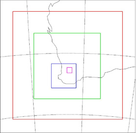Figure 10.  Locations of various grids used in the numerical modeling experiments.

To properly simulate the effects of land surface heterogeneity on regional climate, a realistic representation of surface vegetation characteristics and their seasonal variation are needed.  We will use the MODIS derived vegetation characteristics for this purpose.  Two of the important vegetation characteristics used in the LEAF-2 soil vegetation model within RAMS are Leaf Area Index (LAI) and fractional vegetation cover.  The MODIS-derived LAI product at 1 km resolution is available at both one-and eight-day intervals.  We will use the eight-day interval LAI product to specify seasonal variation of this vegetation characteristic within RAMS.  Fractional vegetation cover is currently not a standard MODIS product.  However, we plan to use NDVI derived from MODIS to specify fractional vegetation cover in RAMS.  We will use the technique outlined in section 5.2 for this purpose.  The MODIS-derived NDVI product is available at a spatial and temporal resolution of 1km and 16 days, respectively. 

<--top

Long-term simulation of clouds

In this set of simulations, we will use a grid with 3km spacing straddling the bunny fence to examine cloud formation along the border region between areas of contrasting land use.  Configuration and locations of grids to be used in these simulations are given in Table 1 and Figure 10.  We will use a procedure similar to that used for simulations RC1 and RC2 utilizing MODIS data to specify current and pristine land use scenarios.  NCEP reanalysis data along with radiosonde observations will be utilized for initializing and forcing the lateral boundaries.  Explicit representation of cloud microphysics will be used to simulate cloud formation for the months of August (LCA1, LCA2: current and pristine scenarios) and January (LCJ1, LCJ2). In these simulations MODIS derived fractional soil moisture will be used to nudge the evolution of surface soil moisture distribution to be consistent with satellite observations. These simulations will be analyzed to determine differences in cloud cover, timing of convection, location of cloud formation, cloud thickness, cloud top and base heights, cloud liquid water content and cloud liquid water path.  The model simulations for the current land use scenario will be compared to GMS observations of cloud cover and cloud location and MODIS derived cloud liquid water path of clouds forming on the either side of the bunny fence.

Specific case studies of cloud formation

We will use numerical modeling simulations with grid spacing less than 1km to examine specific cases of cloud formation in the bunny fence area.  These simulations will focus on days for which land surface characteristics may exert an exceptionally strong influence on cloud formation.  We will consider cases that fall into one of the three categories identified in section 5.6.  If possible, the case study days will be selected to coincide with the field campaigns during which radiosonde observations will be available over adjacent regions on either side of the bunny fence.  We will examine the cloud formation for these selected days with both current and pristine land use scenarios.  We will use a strategy similar to the ones used in simulations described in the previous sections to specify land surface characteristics for current and pristine land use scenarios.  We will use ASTER imagery to specify soil moisture variability at smaller scales to be used in these simulations.  Explicit representation of cloud microphysics will be used in these simulations.

These higher spatial resolution simulations incorporating both satellite and ground based observations will be used explore if the nature of land use and landscape heterogeneity is responsible for preferential cloud formation and triggering of convection along the bunny fence. If they do play an important role, then we will examine the processes though which land use and landscape heterogeneity interact with the formation of convective clouds.  Also we expect these simulations to help us understand environmental conditions under which land use and landscape heterogeneity effects have a significant impact on atmospheric processes. This knowledge will help us estimate the frequency of occurrence of such environmental conditions and thus evaluate the importance of land surface heterogeneity effects on atmospheric convection.

<--top